DataFrames and Pandas
: From Dictionaries to Data Analysis

March 7, 2026
Recap of Previous Lecture
- Maths and operators
- How to assign variables, lists
- For loops
- Conditional statements (
if,elif,else) - Spacing is important!
Today’s Lecture
- Dictionaries
- Introduction to
pandas - Reading the Auckland pedestrian data
- Exploring and filtering DataFrames
- The importance of
.copy() - Groupby and Aggregation
- Reshaping data (Melt and Pivot)
- Merging DataFrames
- Quick Visualisation
What will we “really” cover this week?
- How do we store structured data beyond lists?
- How to import real-world spreadsheet data with
pandas - How to clean, explore, filter, and group data
- How does this connect to geospatial analysis later?
Part 1: Dictionaries
Dictionaries
- A dictionary is another type of variable
- It uses a key:value structure
- Denoted using curly brackets
{} - Useful for storing loosely structured information
- Often combined with lists
Example
city_pop = {
    "Auckland": 1672000,
    "Wellington": 217200,
    "Christchurch": 389700,
    "Hamilton": 185000,
    "Tauranga": 158000
}

city_pop["Auckland"] # 1672000- Compare with a list:
cities[0](access by position) - A dictionary:
city_pop["Auckland"](access by key)
Dictionary Methods
mydict.keys()gives you all the keysmydict.values()gives you all the valuesmydict.items()gives you key-value pairs
Iterating Through Dictionaries
Remember for loops from last week?
Auckland: 1,672,000
Wellington: 217,200
Christchurch: 389,700
Hamilton: 185,000
Tauranga: 158,000
Nested Dictionaries
Dictionaries can contain other dictionaries:
Why Use Dictionaries?
- Dictionaries create more freedom in data structure than lists
- Unlike arrays, they handle mixed data types and uneven structures well
- This matters for ‘semi-structured’ data from the web (e.g. GeoJSON, API responses)
- Some records have geolocation, some do not
- Using a dictionary does not mean no structure, just that not all elements need to be present
Dictionaries and GeoJSON
GeoJSON, the web standard for geographic data, is built on dictionaries:
When you fetch data from LINZ or OpenStreetMap APIs, you get dictionaries like this!
Your Turn (5 min)
The dictionary below has already been created for you:
- Print the count for
"Queen Street"using its key - Add a new sensor:
"Wynyard Quarter"with a count of4800 - Print all sensor names using
sensors.keys()
Part 2: Getting Started with Pandas
Python Packages
- Python’s power comes from packages (libraries)
- Thousands of packages exist for different purposes
- For data analysis and GIS, you will use:
pandas,numpy,matplotlib,geopandas
Installation
How Imports Work
There are three main ways to bring a package into your code:
1. Import the whole package
2. Import with an alias (as)
3. Import specific functions (from)
Standard Aliases
The Python community has agreed on these nicknames:
| Package | Alias | Usage |
|---|---|---|
pandas |
pd |
import pandas as pd |
numpy |
np |
import numpy as np |
matplotlib.pyplot |
plt |
import matplotlib.pyplot as plt |
seaborn |
sns |
import seaborn as sns |
geopandas |
gpd |
import geopandas as gpd |
Using these aliases makes your code readable to other Python users.
from for Specific Items
When you only need one or two things from a package:
# Import just the Path class from pathlib
from pathlib import Path

# Import specific functions
from math import sqrt, pi

print(sqrt(16))   # 4.0
print(pi)         # 3.14159...
When to use from:
- You only need one or two items from a large package
- The item name is clear enough on its own (e.g.
Path,sqrt) - Avoid
from pandas import *as it imports everything and clutters your namespace
What is a DataFrame?
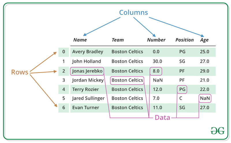
source: geeksforgeeks.org
- Tabular array (like a spreadsheet)
- Rows = observations, Columns = variables
- Think of it as an attribute table without the geometry column (that comes with GeoPandas)
A Toy DataFrame
   a  b
0  1  5
1  2  6
2  3  7
3  4  8
From Dictionary to DataFrame
This is where dictionaries and DataFrames connect:
city_data = {
    'city': ['Auckland', 'Wellington', 'Christchurch'],
    'population': [1672000, 217200, 389700],
    'area_km2': [1086, 444, 608]
}

cities_df = pd.DataFrame(city_data)
print(cities_df)
city population area_km2
0 Auckland 1672000 1086
1 Wellington 217200 444
2 Christchurch 389700 608Each dictionary key becomes a column name.
DataFrame vs Series?
- A Series is 1-dimensional (a single column)
- A DataFrame is 2-dimensional (a table of columns)

Part 3: The Auckland Pedestrian Data
Reading the Data
We have hourly pedestrian counts from 20 sensor locations across Auckland CBD in 2024.
import pandas as pd

ped = pd.read_csv('https://raw.githubusercontent.com/dataandcrowd/GISCI343/refs/heads/main/pedestrians/akl_ped-2024.csv')
print(ped.shape)
(8796, 23)- ~8,800 rows (one per hour per day)
- 23 columns: Date, Time, and 20 sensor locations
- This is wide format: each location is its own column
Understanding the Structure
Always start with .info() and .dtypes to check:
- How many rows and columns?
- Which columns have missing values?
- Are data types correct (numeric vs string)?
.head() and .tail() show the first/last rows.
Column Names
['Date', 'Time', '107 Quay Street', 'Te Ara Tahuhu Walkway',
 'Commerce Street West', '7 Custom Street East', '45 Queen Street',
 '30 Queen Street', '19 Shortland Street', '2 High Street',
 '1 Courthouse Lane', '61 Federal Street', '59 High Street',
 '210 Queen Street', '205 Queen Street', '8 Darby Street EW',
 '8 Darby Street NS', '261 Queen Street', '297 Queen Street',
 '150 K Road', '183 K Road',
 '188 Quay Street Lower Albert (EW)',
 '188 Quay Street Lower Albert (NS)', ...]
These are real sensor locations in Auckland’s city centre.
Summary Statistics
count: how many non-null values (first check for missing data)meanandstd: central tendency and spreadmin,25%,50%,75%,max: the five-number summary- Which locations see the most foot traffic?
Part 4: Selecting and Filtering
Selecting Columns
# Single column (returns a Series)
queen_st = ped['45 Queen Street']

# Single column (returns a DataFrame)
queen_st_df = ped[['45 Queen Street']]

# Multiple columns
subset = ped[['Date', 'Time', '45 Queen Street', '150 K Road']]
Single brackets ['col'] returns a Series; double brackets [['col']] returns a DataFrame.
loc and iloc
.loc[]: label-based selection.iloc[]: integer position-based selection
# iloc: by position
ped.iloc[0:5, 0:4]  # First 5 rows, first 4 columns

# loc: by label
ped.loc[0:2, ['Date', 'Time', '45 Queen Street']]
Key difference:
.iloc[0:3]returns rows 0, 1, 2 (excludes 3).loc[0:3]returns rows 0, 1, 2, 3 (includes 3)
Boolean Indexing (Filtering)
Uses conditionals from last lecture:
# Hours where Queen Street had > 500 pedestrians
busy = ped[ped['45 Queen Street'] > 500]

# Multiple conditions (AND) - use &
both_busy = ped[
    (ped['45 Queen Street'] > 500) &
    (ped['150 K Road'] > 200)
]

# Multiple conditions (OR) - use |
waterfront = ped[
    (ped['107 Quay Street'] > 300) |
    (ped['Te Ara Tahuhu Walkway'] > 300)
]
The query() Method
Cleaner syntax for filtering (column names with spaces need backticks):
Filtering by Date and Time
# Ensure Date is datetime
ped['Date'] = pd.to_datetime(ped['Date'])

# Filter for March 2024
march = ped[ped['Date'].dt.month == 3]

# Weekdays only (Monday=0 to Friday=4)
weekdays = ped[ped['Date'].dt.dayofweek < 5]

# Morning peak hours
morning_peak = ped[ped['Time'].isin(['7:00-7:59', '8:00-8:59', '9:00-9:59'])]
Your Turn (3 min)
Using the pedestrian data:
- Select only the
Date,Time, and45 Queen Streetcolumns - Filter for rows where
45 Queen Street> 300 - Filter for weekend data only (Saturday and Sunday)
- How many rows does each filter produce?
Part 5: Don’t Forget .copy()
The Problem
Assignment in Python creates a reference, not a copy:
pandas_df_new = pandas_df   # NOT a copy!
pandas_df_new['d'] = [13, 14, 15, 16]

print(pandas_df)  # The original is also modified!
a b d
0 1 5 13
1 2 6 14
2 3 7 15
3 4 8 16Both variables point to the same object in memory.
The Solution: .copy()
pandas_df_new = pandas_df.copy()  # A true, independent copy
pandas_df_new['d'] = [13, 14, 15, 16]

print(pandas_df)      # Unchanged!
print(pandas_df_new)  # Only this one has column 'd'
Rule of thumb: if you plan to modify a filtered or sliced DataFrame, always call .copy() first.
Your Turn (3 min)
- Create a toy DataFrame:
pd.DataFrame({'a': [1,2,3,4], 'b': [5,6,7,8]}) - Copy it using
.copy()and assign aspandas_df_new - Add a column
'c'with values[9, 10, 11, 12]to the copy - Print both DataFrames and confirm the original is unchanged
Part 6: Manipulating Data
Creating New Columns
df = ped.copy()
df['Date'] = pd.to_datetime(df['Date'])

# Extract temporal features
df['Month'] = df['Date'].dt.month
df['DayOfWeek'] = df['Date'].dt.day_name()
df['IsWeekend'] = df['Date'].dt.dayofweek >= 5

# Extract the starting hour from the Time string
df['Hour'] = df['Time'].str.split(':').str[0].astype(int)

# Total pedestrians across all sensors
location_cols = df.columns[2:22]
df['Total'] = df[location_cols].sum(axis=1)
Conditional Columns
Using .apply() with a custom function:
def time_of_day(hour):
    if hour < 7:
        return 'Early Morning'
    elif hour < 10:
        return 'Morning Peak'
    elif hour < 16:
        return 'Midday'
    elif hour < 19:
        return 'Evening Peak'
    else:
        return 'Night'

df['Period'] = df['Hour'].apply(time_of_day)
Or using np.where() for binary classification:
Part 7: Groupby and Aggregation
The Split-Apply-Combine Pattern

Source: Soner Yildirim, Towards Data Science
- Split data into groups based on some criterion
- Apply a function to each group independently
- Combine the results into a new data structure
Basic Groupby
# Average pedestrian count on Queen Street by day of week
df.groupby('DayOfWeek')['45 Queen Street'].mean()
DayOfWeek
Friday 285.3
Monday 270.1
Saturday 310.5
Sunday 195.2
Thursday 278.9
Tuesday 265.4
Wednesday 272.8Multiple Aggregations
Grouping by Multiple Variables
# Average count by day of week AND time period
cross_tab = df.groupby(['DayOfWeek', 'Period'])['45 Queen Street'].mean().round(1)

# Unstack for readability (rows = days, columns = periods)
cross_tab.unstack()
This is essentially a cross-tabulation: how does foot traffic vary by both day and time?
Your Turn (5 min)
- Calculate the average hourly count at
45 Queen Streetby month - Which month has the highest average?
- Calculate the total annual count for each of the 20 sensor locations
- Which location is the busiest?
Part 8: Reshaping Data
Melt and Cast
melt(): wide to long formatpivot()/pivot_table(): long to wide format
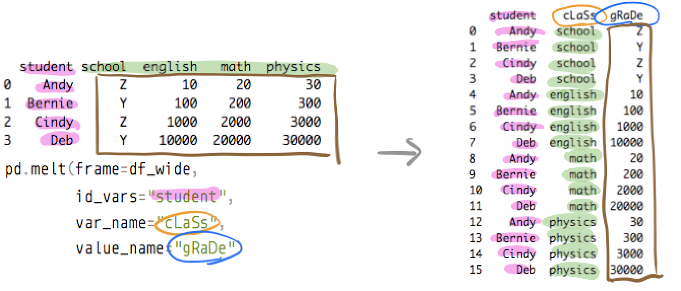
Melt: Wide to Long
The pedestrian data has 20 location columns. We can “melt” them into two columns: Location and Count.
ped_long = df.melt(
    id_vars=['Date', 'Time', 'Hour', 'Month', 'DayOfWeek', 'IsWeekend', 'Period'],
    value_vars=location_cols,
    var_name='Location',
    value_name='Count'
)

print(f"Wide shape: {df.shape}")
print(f"Long shape: {ped_long.shape}")
Wide shape: (8796, 30)
Long shape: (175920, 9)8,796 rows x 20 locations = 175,920 rows
Pivot Table: Long to Wide
# Average hourly count by location and time period
pivot = ped_long.pivot_table(
    values='Count',
    index='Location',
    columns='Period',
    aggfunc='mean'
).round(1)

print(pivot)
Rule of thumb: making a table? Pivot. Making a plot? Melt.
Part 9: Handling Missing Data
Detecting Missing Values
Filling Missing Values
Different approaches for different situations:
# Fill with zero (sensor was working, no one walked by)
ped_zero = ped.fillna(0)

# Fill with column mean (sensor was temporarily offline)
ped_mean = ped.copy()
ped_mean['45 Queen Street'] = ped_mean['45 Queen Street'].fillna(
    ped_mean['45 Queen Street'].mean()
)

# Forward fill (use previous hour's value for brief gaps)
ped_ffill = ped.fillna(method='ffill')

# Interpolation (best for time series)
ped_interp = ped.copy()
ped_interp['45 Queen Street'] = ped_interp['45 Queen Street'].interpolate(
    method='linear'
)
Think Before You Fill!
- Missing at random (sensor malfunction): safe to fill with mean/interpolation
- Missing systematically (fails during rain): filling naively biases your results
- Missing by design (sensor not yet installed): keep as
NaN, do not fill with zero
Always document what you did and why.
Part 10: Merging DataFrames
Join Types
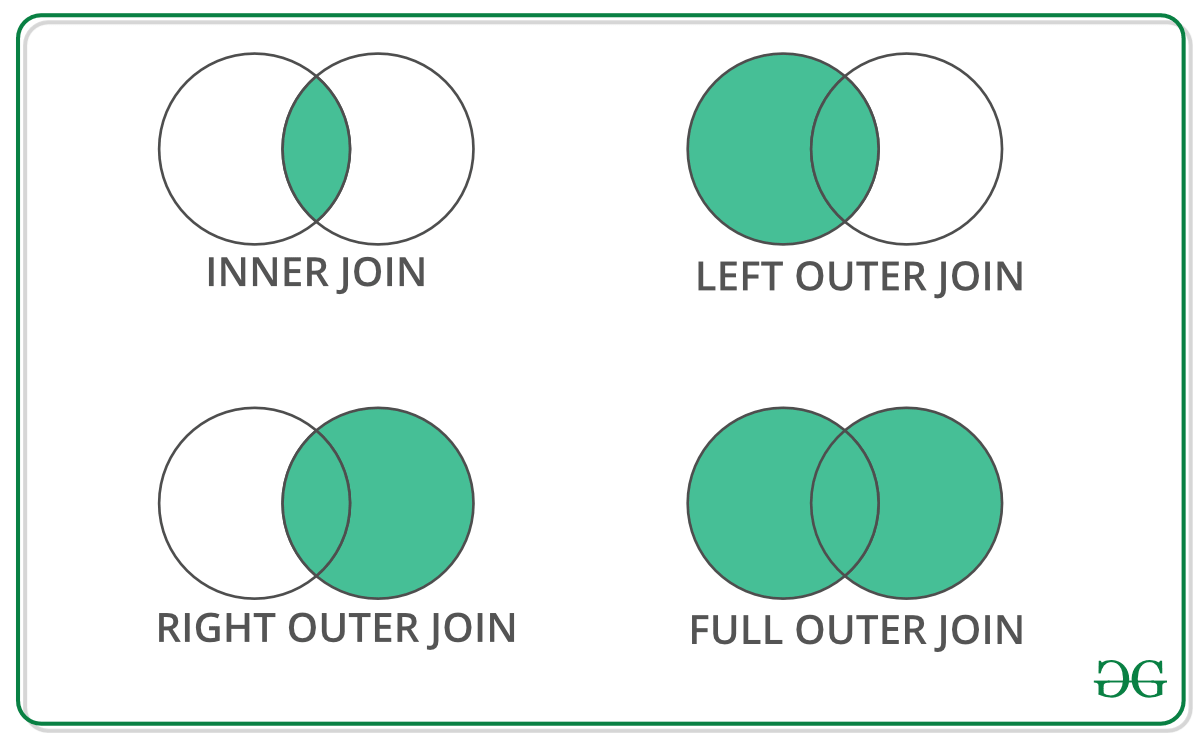
Example: Two DataFrames
Merging
Merging with the Pedestrian Data
Once we melt to long format, we can merge with sensor metadata:
sensor_metadata = pd.DataFrame({
    'Location': ['107 Quay Street', '45 Queen Street', '150 K Road'],
    'Area': ['Waterfront', 'CBD', 'K Road'],
    'Latitude': [-36.8430, -36.8442, -36.8580],
    'Longitude': [174.7685, 174.7659, 174.7560]
})

merged = pd.merge(ped_long, sensor_metadata, on='Location', how='inner')
This adds spatial attributes (coordinates, area type) to each pedestrian count record. In Section 2.4, you will do this with geometry using spatial joins in GeoPandas.
Part 11: Quick Visualisation
pandas Plotting
pandas DataFrames have built-in plotting via matplotlib:
import matplotlib.pyplot as plt

# Bar chart of average hourly counts by location
location_means = ped[location_cols].mean().sort_values(ascending=False)
location_means.plot(kind='barh', figsize=(10, 8), color='steelblue')
plt.xlabel('Average Hourly Pedestrian Count')
plt.title('Average Hourly Counts by Sensor Location (2024)')
plt.tight_layout()
plt.show()
Hourly Pattern
# Weekday vs Weekend hourly pattern
weekday_avg = df[~df['IsWeekend']].groupby('Hour')['Total'].mean()
weekend_avg = df[df['IsWeekend']].groupby('Hour')['Total'].mean()

plt.figure(figsize=(10, 5))
plt.plot(weekday_avg.index, weekday_avg.values, marker='o', label='Weekday')
plt.plot(weekend_avg.index, weekend_avg.values, marker='s', label='Weekend')
plt.xlabel('Hour of Day')
plt.ylabel('Total Count (all sensors)')
plt.title('Weekday vs Weekend Pedestrian Patterns')
plt.legend()
plt.grid(True, alpha=0.3)
plt.tight_layout()
plt.show()
We will learn much more about visualisation in the next lecture (Section 2.3).
Summary
- Dictionaries: key-value structures, foundation for GeoJSON and APIs
- pandas DataFrames: Python’s answer to spreadsheets
- Reading data:
pd.read_excel(),pd.read_csv() - Exploring:
.head(),.info(),.describe(),.shape - Filtering: boolean indexing,
.loc[],.iloc[],.query() .copy(): always copy before modifying subsets- Groupby: split-apply-combine for aggregation
- Reshaping:
melt()for wide-to-long,pivot_table()for long-to-wide - Missing data: detect, understand why, then fill appropriately
- Merging:
pd.merge()with inner, left, right, outer joins
Looking Ahead
- Section 2.3: Data Visualisation with matplotlib and seaborn
- Section 2.4: GeoPandas - adding geometry to your DataFrames
- A GeoDataFrame is just a DataFrame with a geometry column
- Every pandas skill you learned today transfers directly
Thanks!
Q & A
![]()