2.2. DataFrames and Pandas

Introduction

In Section 2.1, you learned Python fundamentals: lists for storing sequences, loops for iteration, and conditionals for decision-making. Now we build on those foundations to work with structured tabular data, the kind you encounter in Excel spreadsheets, GIS attribute tables, and pedestrian survey databases.

This section introduces three interconnected concepts. First, dictionaries provide flexible key-value structures that underpin GeoJSON (the web standard for geographic data) and API responses. Second, pandas DataFrames offer Python’s answer to spreadsheets and database tables, providing a powerful and reproducible environment for data manipulation. Third, you will learn the core data operations for reading, filtering, grouping, and transforming datasets.

Understanding why these skills matter requires appreciating the nature of geospatial work. Most spatial analysis involves attribute data alongside geometry. In pedestrian mobility research, for example, you might have a dataset of street segments where each row carries both geometric information (the line representing the street) and attribute data (pedestrian counts, pavement width, land-use classification, accessibility index scores).

Before you can perform spatial operations, you typically need to clean, filter, merge, and transform these attributes. Tabular operations such as aggregating counts by time period, filtering locations by volume thresholds, and reshaping wide data into long format are all prerequisites to the spatial analysis and network modelling that follow in later sections.

To make this concrete, we will work with a real dataset throughout this section: hourly pedestrian counts from 20 sensor locations across Auckland’s city centre in 2024. This is the same kind of data that urban planners, transport engineers, and walkability researchers use to understand how people move through cities. By the end of this section, you will be able to load this dataset, explore its structure, filter it by time and location, compute summary statistics, reshape it for visualisation, and combine it with other data sources.

The progression through Part 2 follows a deliberate logic. Section 2.1 established the basics (lists, loops, conditionals). This section (2.2) introduces structured data handling through dictionaries and DataFrames. Section 2.3 will teach you to visualise these data for pattern detection and communication. Section 2.4 then adds the spatial dimension through GeoPandas, building directly on everything you learn here.

Dictionaries: Flexible Data Structures

What is a Dictionary?

Remember lists from Section 2.1? They store items by position:

cities = ['Auckland', 'Wellington', 'Christchurch']
print(cities[0])  # Auckland

Dictionaries store items by key instead of position:

populations = {
    'Auckland': 1672000,
    'Wellington': 217200,
    'Christchurch': 389700
}
print(populations['Auckland'])  # 1672000

Think of a dictionary as a lookup table: you provide a key, it gives you a value.

Creating Dictionaries

# Simple dictionary - city populations
city_pop = {
    "Auckland": 1672000,
    "Wellington": 217200,
    "Christchurch": 389700,
    "Hamilton": 185000,
    "Tauranga": 158000
}

# Access by key
print(city_pop["Auckland"])  # 1672000

# Add new entry
city_pop["Dunedin"] = 134600

# Modify existing
city_pop["Auckland"] = 1700000  # Updated estimate

# Check if key exists
if "Napier" in city_pop:
    print("Found Napier")
else:
    print("Napier not in dictionary")

Dictionary Methods

# Get all keys
city_pop.keys()
# Output: dict_keys(['Auckland', 'Wellington', ...])

# Get all values
city_pop.values()
# Output: dict_values([1672000, 217200, ...])

# Get key-value pairs
city_pop.items()
# Output: dict_items([('Auckland', 1672000), ...])

# Safe access with default
city_pop.get('Napier', 0)  # Returns 0 if key doesn't exist

Iterating Through Dictionaries

Remember for loops from Section 2.1? They work great with dictionaries:

# Iterate through keys
for city in city_pop.keys():
    print(city)

# Iterate through values
for population in city_pop.values():
    print(f"{population:,}")

# Iterate through both (most common!)
for city, population in city_pop.items():
    print(f"{city}: {population:,}")

Output:

Auckland: 1,672,000
Wellington: 217,200
Christchurch: 389,700
...

Connection to Section 2.1: This uses the same for loop syntax you learned, but now with dictionaries instead of lists!

Nested Dictionaries

Dictionaries can contain other dictionaries or lists. This is where they become powerful:

# Pedestrian sensor metadata for Auckland CBD
sensor_info = {
    "45 Queen Street": {
        "latitude": -36.8442,
        "longitude": 174.7659,
        "installed": 2019,
        "direction": "bidirectional"
    },
    "150 K Road": {
        "latitude": -36.8580,
        "longitude": 174.7560,
        "installed": 2020,
        "direction": "bidirectional"
    },
    "107 Quay Street": {
        "latitude": -36.8430,
        "longitude": 174.7685,
        "installed": 2018,
        "direction": "bidirectional"
    }
}

# Access nested data
print(sensor_info["45 Queen Street"]["latitude"])  # -36.8442

# Iterate through nested structure (using Section 2.1 loops!)
for location, metadata in sensor_info.items():
    print(f"\n{location}:")
    for key, value in metadata.items():
        print(f"  {key}: {value}")

Why Dictionaries Matter for GIS

Dictionaries are Everywhere in GIS

GeoJSON, the web standard for geographic data, is built entirely on dictionaries:

# A GeoJSON point feature (this is a dictionary!)
sensor_feature = {
    "type": "Feature",
    "geometry": {
        "type": "Point",
        "coordinates": [174.7659, -36.8442]  # longitude, latitude
    },
    "properties": {
        "name": "45 Queen Street",
        "installed": 2019,
        "avg_daily_count": 8500
    }
}

# Access the coordinates
coords = sensor_feature["geometry"]["coordinates"]
print(f"Sensor is at {coords[1]}°S, {coords[0]}°E")

# Access properties
print(f"Average daily count: {sensor_feature['properties']['avg_daily_count']:,}")

Why this format? Dictionaries are flexible, so not all features need the same properties. They are web-friendly, because JavaScript uses identical syntax (hence “JSON”). And they support nesting, which keeps geometry and attributes separate but together.

Real-world example: When you fetch data from LINZ Data Service API or OpenStreetMap API, you get dictionaries like this!

Practical Example: API Response

# Simulating an API response for Auckland pedestrian sensors
sensors_api_response = {
    "status": "success",
    "count": 3,
    "features": [
        {
            "name": "45 Queen Street",
            "avg_daily": 8500,
            "type": "infrared",
            "location": {"lat": -36.8442, "lon": 174.7659}
        },
        {
            "name": "150 K Road",
            "avg_daily": 4200,
            "type": "infrared",
            "location": {"lat": -36.8580, "lon": 174.7560}
        },
        {
            "name": "107 Quay Street",
            "avg_daily": 6100,
            "type": "infrared",
            "location": {"lat": -36.8430, "lon": 174.7685}
        }
    ]
}

# Extract sensor names (using Section 2.1 concepts!)
sensor_names = []
for sensor in sensors_api_response["features"]:
    sensor_names.append(sensor["name"])

print("Auckland sensors:", sensor_names)

# Using conditionals (Section 2.1!) to filter
busy_sensors = []
for sensor in sensors_api_response["features"]:
    if sensor["avg_daily"] > 5000:  # Conditional from 2.1!
        busy_sensors.append(sensor["name"])

print("High-traffic sensors:", busy_sensors)

Packages and Imports

Before working with pandas, it is worth understanding how Python’s package system works, since you will use import statements at the top of every script from this point onwards.

Installing Packages

Python’s standard library covers the basics, but most data analysis and geospatial work relies on third-party packages. You install them once, then import them into any script that needs them.

# Using uv (recommended for this course)
# uv add pandas

# Using pip
# pip install pandas

# Using conda
# conda install pandas

The `import` Statement

There are three main ways to bring a package into your code. The first is to import the entire package by name, which requires you to prefix every function call with that name:

import pandas
pandas.read_csv('data.csv')  # Must write "pandas." every time

The second, and most common, is to import with an alias using as. This gives the package a shorter nickname:

import pandas as pd
pd.read_csv('data.csv')  # Shorter and conventional

The third is to import specific items from a package using from, which lets you use them directly without any prefix:

from pathlib import Path
my_path = Path('data/')  # No prefix needed

from math import sqrt, pi
print(sqrt(16))  # 4.0

The from approach is best when you only need one or two items from a package and the names are unambiguous on their own. Avoid from pandas import *, which imports everything into your namespace and makes it unclear where each function comes from.

Standard Aliases

The Python community has settled on conventional aliases for the most common data science packages:

import pandas as pd           # Data manipulation
import numpy as np             # Numerical computing
import matplotlib.pyplot as plt  # Plotting
import seaborn as sns          # Statistical graphics
import geopandas as gpd        # Geospatial data (Section 2.4)

Using these aliases makes your code instantly readable to other Python users. When you see pd.read_csv() in someone else’s code, you know immediately that it is a pandas function.

Getting Started with Pandas

What is pandas?

pandas is Python’s data analysis library. Think of it as “Excel in Python, but more powerful and reproducible.” It provides two primary data structures: a DataFrame, which is a table with rows and columns (like a spreadsheet), and a Series, which is a single column of data. On top of these structures, pandas offers a rich set of operations for filtering, grouping, reshaping, and merging datasets.

The reason pandas matters for geospatial work is that most of what you do with spatial data begins with tabular manipulation. Before you can map pedestrian flows across Auckland, you need to read the data, inspect it for quality issues, filter it to the time periods you care about, and aggregate it by location or hour. pandas handles all of this.

Import

import pandas as pd
import numpy as np  # Often used together

Why pd and not pandas?

Typing pandas.read_csv() dozens of times in a script gets tedious. The alias pd is universally understood in the Python community, so using it signals to readers that you are following standard conventions. The same logic applies to np for numpy, plt for matplotlib, and gpd for geopandas.

Creating DataFrames

What is a DataFrame?

A DataFrame is a two-dimensional table with rows (observations or records), columns (variables or fields), and an index (row labels, usually numbers).

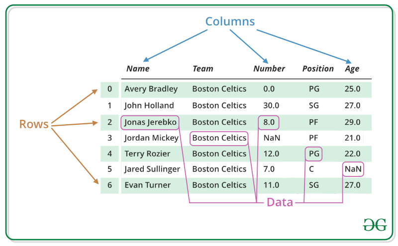
In GIS terms, think of it as an attribute table without the geometry column. That geometry column comes in Section 2.4, when you learn GeoPandas.

From a Dictionary (The Key Connection!)

This is where dictionaries and DataFrames connect. Each dictionary key becomes a column name, and each list of values becomes the column data:

import pandas as pd

# Step 1: Create a dictionary (Section 2.2 beginning!)
city_data = {
    'city': ['Auckland', 'Wellington', 'Christchurch', 'Hamilton', 'Tauranga'],
    'population': [1672000, 217200, 389700, 185000, 158000],
    'area_km2': [1086, 444, 608, 877, 135],
    'region': ['Auckland', 'Wellington', 'Canterbury', 'Waikato', 'Bay of Plenty']
}

# Step 2: Convert to DataFrame
cities_df = pd.DataFrame(city_data)

# Step 3: View it
print(cities_df)

Output:

          city  population  area_km2           region
0     Auckland     1672000      1086         Auckland
1   Wellington      217200       444       Wellington
2  Christchurch      389700       608        Canterbury
3     Hamilton      185000       877          Waikato
4     Tauranga      158000       135  Bay of Plenty

Notice that each dictionary key becomes a column name, each list becomes a column, and pandas automatically adds an index (0, 1, 2, 3, 4).

From a List of Dictionaries

Sometimes data comes as multiple dictionaries (common from APIs):

# Pedestrian sensor locations (like an API might return)
sensors_list = [
    {"name": "45 Queen Street", "avg_daily": 8500, "area": "CBD"},
    {"name": "150 K Road", "avg_daily": 4200, "area": "K Road"},
    {"name": "107 Quay Street", "avg_daily": 6100, "area": "Waterfront"},
    {"name": "Te Ara Tahuhu Walkway", "avg_daily": 3800, "area": "Waterfront"}
]

# Convert to DataFrame
sensors_df = pd.DataFrame(sensors_list)
print(sensors_df)

Output:

                   name  avg_daily        area
0       45 Queen Street       8500         CBD
1          150 K Road       4200      K Road
2     107 Quay Street       6100  Waterfront
3  Te Ara Tahuhu Walkway  3800  Waterfront

This is exactly what you will do with GeoJSON! Each feature becomes a row.

Reading the Auckland Pedestrian Data

Now let us move from toy examples to a real dataset. Throughout the rest of this section, we will work with hourly pedestrian count data collected from 20 sensor locations across Auckland CBD during 2024. This dataset is in wide format: each sensor location is its own column, and each row represents one hour of one day.

Reading a CSV File

import pandas as pd

# Read the Auckland pedestrian count data from GitHub
url = 'https://raw.githubusercontent.com/dataandcrowd/GISCI343/refs/heads/main/pedestrians/akl_ped-2024.csv'
ped = pd.read_csv(url)

# Quick look at the first few rows
print(ped.head())

The pd.read_csv() function reads comma-separated values into a DataFrame. You can pass it a local file path or a URL, which makes it straightforward to load data hosted on GitHub or other repositories. The function accepts many useful arguments, including sep for specifying the delimiter, skiprows for skipping metadata rows, and usecols for selecting specific columns.

Other File Formats

pandas can read many file formats beyond CSV. The most common ones you will encounter in geospatial work are:

# Local CSV file
df = pd.read_csv('data.csv')

# Tab-separated files
df = pd.read_csv('data.txt', sep='\t')

# JSON (common from APIs and GeoJSON)
df = pd.read_json('data.json')

# Excel files (requires openpyxl)
df = pd.read_excel('data.xlsx')

Common arguments that work across most read_ functions include skiprows for skipping header metadata, header for specifying which row contains column names, dtype for setting column data types, na_values for defining what counts as missing data, parse_dates for converting date strings to datetime objects, usecols for selecting specific columns, and nrows for reading only the first n rows.

Saving DataFrames

# Save to CSV (most portable)
df.to_csv('output.csv', index=False)  # index=False avoids an extra column

# Save to Excel (requires openpyxl)
# df.to_excel('output.xlsx', sheet_name='Data', index=False)

# Save to JSON
df.to_json('output.json', orient='records', indent=2)

Exploring the Pedestrian Data

Once you have loaded a dataset, the first step is always to understand its structure, size, and quality. Let us explore the Auckland pedestrian data.

Initial Inspection

# View first 5 rows
print(ped.head())

# View last 5 rows
print(ped.tail())

# View 3 random rows
print(ped.sample(3))

The .head() and .tail() methods let you see the beginning and end of your data. The .sample() method selects random rows, which is useful for spotting patterns that might not appear at the top or bottom of a sorted dataset.

DataFrame Properties

# Shape: (rows, columns)
print(ped.shape)  # (8796, 23) approximately

# Column names
print(ped.columns.tolist())

Output:

['Date', 'Time', '107 Quay Street', 'Te Ara Tahuhu Walkway',
 'Commerce Street West', '7 Custom Street East', '45 Queen Street',
 '30 Queen Street', '19 Shortland Street', '2 High Street',
 '1 Courthouse Lane', '61 Federal Street', '59 High Street',
 '210 Queen Street', '205 Queen Street', '8 Darby Street EW',
 '8 Darby Street NS', '261 Queen Street', '297 Queen Street',
 '150 K Road', '183 K Road',
 '188 Quay Street Lower Albert (EW)',
 '188 Quay Street Lower Albert (NS)', ...]

Notice the structure: each row is one hour of one day, and each location has its own column. This wide format is common in sensor data but, as you will learn later in this section, is not always the best shape for analysis or visualisation.

Data Types

# Check data types of each column
print(ped.dtypes)

The Date column should be a datetime type (or object if not yet parsed), Time is a string (e.g. “6:00-6:59”), and the location columns should be numeric (int64 or float64). If any numeric column shows up as object, that usually means there are non-numeric entries (such as text notes or error codes) that need cleaning.

Information Summary

# Comprehensive overview
print(ped.info())

The .info() method provides a structural overview of your DataFrame: the total number of rows and columns, which columns contain missing values (indicated by a non-null count less than the total row count), the data type of each column, and the memory footprint. This is typically the first method you should call when working with a new dataset, because it immediately flags potential issues such as numeric columns stored as strings or unexpected null values.

Summary Statistics

# Summary statistics for all numeric columns
print(ped.describe())

The .describe() output provides a concise statistical profile of each numeric column. The count row tells you how many non-null values exist, which is your first check for missing data. The mean and std (standard deviation) rows summarise the central tendency and spread of the distribution. The five-number summary (min, 25%, 50%, 75%, max) describes the distribution’s shape, with the 50% row representing the median. For the pedestrian data, these statistics immediately reveal which locations see the most foot traffic and whether any sensors have unusually low counts that might indicate downtime.

Custom statistics for a single column:

# Statistics for one sensor location
print(ped['45 Queen Street'].mean())    # Average hourly count
print(ped['45 Queen Street'].median())  # Median hourly count
print(ped['45 Queen Street'].max())     # Peak hourly count
print(ped['45 Queen Street'].sum())     # Total annual count

# Multiple statistics at once
print(ped['45 Queen Street'].agg(['mean', 'median', 'min', 'max', 'std']))

Selecting Data

Selecting Columns

# Single column (returns a Series)
queen_st = ped['45 Queen Street']
print(type(queen_st))  # <class 'pandas.core.series.Series'>

# Single column (returns a DataFrame)
queen_st_df = ped[['45 Queen Street']]
print(type(queen_st_df))  # <class 'pandas.core.frame.DataFrame'>

# Multiple columns
subset = ped[['Date', 'Time', '45 Queen Street', '150 K Road']]
print(subset.head())

The difference between single brackets ped['col'] (returns a Series) and double brackets ped[['col']] (returns a DataFrame) matters when chaining operations, because some methods behave differently on Series vs DataFrame objects.

Selecting Rows by Index

Using .iloc[] (integer location) selects rows and columns by their numeric position:

# First row
first_row = ped.iloc[0]
print(first_row)

# First 5 rows, first 4 columns
subset = ped.iloc[0:5, 0:4]
print(subset)

# Specific rows
selected = ped.iloc[[0, 100, 500]]
print(selected)

Using .loc[] (label-based) selects by index label and column name:

# Row with index label 0
row = ped.loc[0]

# First 3 rows, specific columns
subset = ped.loc[0:2, ['Date', 'Time', '45 Queen Street']]
print(subset)

The key difference is that .iloc[0:3] returns rows 0, 1, 2 (excludes 3), while .loc[0:3] returns rows 0, 1, 2, 3 (includes 3 if it exists). This can be confusing at first, so pay attention to which one you are using.

Boolean Indexing (Filtering)

This is the most powerful selection method. It uses the conditionals from Section 2.1 to create a True/False mask that filters rows.

# Find hours where Queen Street had more than 500 pedestrians
busy_hours = ped[ped['45 Queen Street'] > 500]
print(f"Hours with >500 pedestrians on Queen St: {len(busy_hours)}")

# Find hours where K Road was quiet (fewer than 50 pedestrians)
quiet_krd = ped[ped['150 K Road'] < 50]
print(f"Quiet hours on K Road: {len(quiet_krd)}")

# Multiple conditions (AND) - use &
# Busy Queen Street AND busy K Road at the same time
both_busy = ped[
    (ped['45 Queen Street'] > 500) &
    (ped['150 K Road'] > 200)
]
print(f"Hours where both locations were busy: {len(both_busy)}")

# Multiple conditions (OR) - use |
# Either waterfront location is busy
waterfront_busy = ped[
    (ped['107 Quay Street'] > 300) |
    (ped['Te Ara Tahuhu Walkway'] > 300)
]
print(f"Hours with busy waterfront: {len(waterfront_busy)}")

Filtering by Date and Time

The pedestrian data includes Date and Time columns, which allow temporal filtering:

# Clean non-data rows first, then convert Date to datetime
ped = ped.dropna(subset=['Date', 'Time'])
ped = ped[ped['Date'] != 'Daylight Savings']
ped['Date'] = pd.to_datetime(ped['Date'])

# Filter for a specific month (e.g. March 2024)
march = ped[ped['Date'].dt.month == 3]
print(f"March rows: {len(march)}")

# Filter for a specific day of the week (0 = Monday, 6 = Sunday)
weekdays = ped[ped['Date'].dt.dayofweek < 5]  # Monday to Friday
weekends = ped[ped['Date'].dt.dayofweek >= 5]  # Saturday and Sunday

print(f"Weekday rows: {len(weekdays)}")
print(f"Weekend rows: {len(weekends)}")

# Filter for morning peak hours (using the Time string column)
morning_peak = ped[ped['Time'].isin(['7:00-7:59', '8:00-8:59', '9:00-9:59'])]
print(f"Morning peak rows: {len(morning_peak)}")

The `.query()` Method

The .query() method provides a cleaner syntax for filtering, especially with complex conditions:

# Simple condition
busy = ped.query('`45 Queen Street` > 500')

# Note: column names with spaces need backticks in .query()
# Multiple conditions
peak = ped.query('`45 Queen Street` > 500 and `150 K Road` > 200')

# Using variables (with @)
threshold = 300
high_traffic = ped.query('`107 Quay Street` > @threshold')

Copying DataFrames

References vs Copies

One common source of bugs in pandas is the distinction between a reference and a copy. When you assign a subset of a DataFrame to a new variable, pandas sometimes creates a reference (a view into the original data) rather than an independent copy. This means that modifying the new variable can unintentionally modify the original.

# This might create a reference, not a copy
subset = ped[ped['Date'].dt.month == 3]

# To be safe, always use .copy() when you plan to modify a subset
march_data = ped[ped['Date'].dt.month == 3].copy()

# Now you can safely modify march_data without affecting ped
march_data['total'] = march_data['45 Queen Street'] + march_data['150 K Road']

The rule of thumb is: if you plan to modify a filtered or sliced DataFrame, always call .copy() first. This avoids the SettingWithCopyWarning that pandas raises when it detects potentially ambiguous assignments. This is a small habit that prevents frustrating debugging sessions later.

Manipulating Data

Creating New Columns

Working with the pedestrian data, you will often need to derive new variables from existing ones:

# Make a working copy
df = ped.copy()

# Ensure Date is datetime
df['Date'] = pd.to_datetime(df['Date'])

# Extract useful temporal features
df['Month'] = df['Date'].dt.month
df['DayOfWeek'] = df['Date'].dt.day_name()  # 'Monday', 'Tuesday', etc.
df['IsWeekend'] = df['Date'].dt.dayofweek >= 5  # True/False

# Extract the starting hour from the Time string (e.g. "7:00-7:59" -> 7)
df['Hour'] = df['Time'].str.split(':').str[0].astype(int)

# Calculate total pedestrians across all sensors for each hour
location_cols = df.columns[2:22]  # The 20 sensor columns
df['Total'] = df[location_cols].sum(axis=1)

# Calculate the mean across all sensors for each hour
df['Mean'] = df[location_cols].mean(axis=1)

print(df[['Date', 'Time', 'Hour', 'DayOfWeek', 'IsWeekend', 'Total']].head(10))

Conditional Column Creation

You can create categorical columns using functions and .apply():

# Classify hours by time of day
def time_of_day(hour):
    if hour < 7:
        return 'Early Morning'
    elif hour < 10:
        return 'Morning Peak'
    elif hour < 16:
        return 'Midday'
    elif hour < 19:
        return 'Evening Peak'
    else:
        return 'Night'

df['Period'] = df['Hour'].apply(time_of_day)
print(df[['Time', 'Hour', 'Period']].drop_duplicates())

You can also use np.where() for simple binary classifications:

import numpy as np

# Classify Queen Street hours as busy or quiet
df['QueenSt_Busy'] = np.where(df['45 Queen Street'] > 300, 'Busy', 'Quiet')

Modifying and Renaming Columns

# Rename columns for easier access
df = df.rename(columns={
    '45 Queen Street': 'queen_st_45',
    '150 K Road': 'k_road_150',
    '107 Quay Street': 'quay_st_107'
})

# Drop unnecessary columns
df = df.drop(columns=['Mean'])  # If you no longer need it

# Reset the index after filtering
filtered = df[df['Month'] == 1].reset_index(drop=True)

Grouping and Aggregation

Grouping is one of the most powerful features in pandas. It follows the split-apply-combine pattern: split the data into groups based on some criterion, apply a function to each group independently, and combine the results into a new DataFrame. In the pedestrian data context, this is how you answer questions like “what is the average hourly count at each location?” or “which day of the week sees the most foot traffic?”

Basic Grouping

# Average pedestrian count on Queen Street by day of the week
daily_avg = df.groupby('DayOfWeek')['queen_st_45'].mean()
print(daily_avg)

Output:

DayOfWeek
Friday       285.3
Monday       270.1
Saturday     310.5
Sunday       195.2
Thursday     278.9
Tuesday      265.4
Wednesday    272.8
Name: queen_st_45, dtype: float64

Multiple Aggregations

# Multiple statistics for Queen Street by day of week
queen_st_stats = df.groupby('DayOfWeek')['queen_st_45'].agg(
    ['mean', 'median', 'max', 'count']
)
print(queen_st_stats)

Aggregating Multiple Columns

# Compare multiple locations by time period
period_summary = df.groupby('Period').agg({
    'queen_st_45': ['mean', 'max'],
    'k_road_150': ['mean', 'max'],
    'quay_st_107': ['mean', 'max']
}).round(1)

print(period_summary)

Grouping by Multiple Variables

You can group by more than one column to create cross-tabulations:

# Average pedestrian count by day of week AND time period
cross_tab = df.groupby(['DayOfWeek', 'Period'])['queen_st_45'].mean().round(1)
print(cross_tab)

# Unstack to make it more readable (rows = days, columns = periods)
cross_tab_wide = cross_tab.unstack()
print(cross_tab_wide)

Custom Aggregation Functions

# Define a custom function: range of values
def count_range(values):
    return values.max() - values.min()

# Apply it in groupby
daily_range = df.groupby('DayOfWeek')['queen_st_45'].agg([
    'mean',
    ('range', count_range),
    'count'
])
print(daily_range)

Practical Example: Monthly Pedestrian Volumes

# Total monthly pedestrians at each location
monthly_totals = df.groupby('Month')[location_cols].sum()
print(monthly_totals)

# Which month had the highest total foot traffic across all sensors?
monthly_grand_total = monthly_totals.sum(axis=1)
busiest_month = monthly_grand_total.idxmax()
print(f"\nBusiest month: {busiest_month} with {monthly_grand_total.max():,.0f} total counts")

Reshaping Data

The Auckland pedestrian data arrives in wide format: each sensor location is a separate column. This is convenient for some analyses but not for others. Understanding when and how to reshape data between wide and long formats is an essential skill.

Melting (Wide to Long)

The melt() function converts wide data to long format by “unpivoting” columns into rows. This is exactly what the pedestrian data needs for most visualisation and many analysis tasks:

# Melt the pedestrian data from wide to long format
ped_long = df.melt(
    id_vars=['Date', 'Time', 'Hour', 'Month', 'DayOfWeek', 'IsWeekend', 'Period'],
    value_vars=location_cols,
    var_name='Location',
    value_name='Count'
)

print(ped_long.head(10))
print(f"\nWide shape: {df.shape}")
print(f"Long shape: {ped_long.shape}")

Output:

        Date       Time  Hour  Month DayOfWeek  IsWeekend      Period  \
0 2024-01-01  6:00-6:59     6      1    Monday      False  Early Morning
1 2024-01-01  7:00-7:59     7      1    Monday      False  Morning Peak
...

          Location  Count
0  107 Quay Street     12
1  107 Quay Street     45
...

Wide shape: (8796, 30)
Long shape: (175920, 9)

The wide format had ~8,800 rows with 20 location columns. The long format has ~176,000 rows (8,800 x 20) but only one Location column and one Count column. The long format is far more natural for operations like “compare the average count across all locations” or “plot counts over time coloured by location.”

Pivot Tables (Long to Wide)

The pivot_table() function does the reverse, converting long data back to wide format, optionally with aggregation:

# Average hourly count by location and time period
pivot = ped_long.pivot_table(
    values='Count',
    index='Location',
    columns='Period',
    aggfunc='mean'
).round(1)

print(pivot)

This produces a table where each row is a sensor location and each column is a time period, with average hourly counts in the cells. This wide format is ideal for quick comparison across categories.

When to Use Which Format

Knowing when to pivot and when to melt depends on your goal. Pivot tables are best for analysis and comparison, because having categories as columns makes it easy to scan values across groups (e.g. morning vs. evening pedestrian counts at different locations). Melting is best for visualisation, because most plotting libraries (matplotlib, seaborn, plotly) expect data in long format where each observation occupies its own row. A good rule of thumb: if you are making a table, pivot; if you are making a plot, melt.

Handling Missing Data

Real-world sensor data is messy. Sensors malfunction, get obscured, or lose power. The Auckland pedestrian data almost certainly contains missing values or zeros where counts should exist.

Detecting Missing Data

# Check for missing values across the entire DataFrame
print(ped.isnull().sum())

# Total missing values
print(f"\nTotal missing values: {ped.isnull().sum().sum()}")

# Percentage missing per column
missing_pct = (ped.isnull().sum() / len(ped) * 100).round(2)
print(missing_pct[missing_pct > 0])  # Show only columns with missing data

Removing Missing Data

# Drop rows where ANY value is missing
clean = ped.dropna()
print(f"Rows before: {len(ped)}, after: {len(clean)}")

# Drop rows where a specific column is missing
clean = ped.dropna(subset=['45 Queen Street'])

# Drop columns where ANY value is missing
clean = ped.dropna(axis=1)

Filling Missing Data

Each of the following approaches suits a different situation. Choose the one that matches why your data is missing:

# Fill with zero (appropriate if missing means "no pedestrians detected")
ped_zero = ped.fillna(0)

# Fill with column mean (appropriate if sensor was temporarily offline)
ped_mean = ped.copy()
ped_mean['45 Queen Street'] = ped_mean['45 Queen Street'].fillna(
    ped_mean['45 Queen Street'].mean()
)

# Forward fill (use the previous hour's value - good for brief sensor gaps)
ped_ffill = ped.fillna(method='ffill')

# Backward fill (use the next hour's value)
ped_bfill = ped.fillna(method='bfill')

# Linear interpolation (best for time series with short gaps)
ped_interp = ped.copy()
ped_interp['45 Queen Street'] = ped_interp['45 Queen Street'].interpolate(
    method='linear'
)

Best Practices

Handling Missing Data Thoughtfully

Before removing or filling missing values, you should understand why they are missing. Data that is missing at random (e.g. a pedestrian sensor that happened to malfunction one afternoon) is generally safe to fill with a mean or interpolated value. Data that is missing systematically (e.g. a sensor that consistently fails during heavy rain, precisely when pedestrian patterns change most) requires investigation because filling it naively could bias your results. Data that is missing by design (e.g. a sensor that was not yet installed at the start of the year) should typically remain as NaN rather than being filled with zero, because zero implies “we observed no pedestrians” while NaN correctly states “we have no observation.”

Whatever approach you choose, document it explicitly in your code or analysis report. Consider creating a binary indicator column (e.g. queen_st_was_missing) so that downstream analyses can account for imputed values. Always report how many values were handled and by which method.

In geospatial contexts specifically, missing coordinates or key spatial identifiers usually mean you must drop the record, because there is no meaningful way to impute a location. Missing attributes, by contrast, can often be filled using spatial neighbours (a technique you will encounter in more advanced spatial analysis) or statistical methods.

Merging DataFrames

Combining datasets is essential for analysis. In the pedestrian data context, you might want to merge the count data with sensor location metadata (coordinates, street type, nearest land use) to enable spatial analysis.

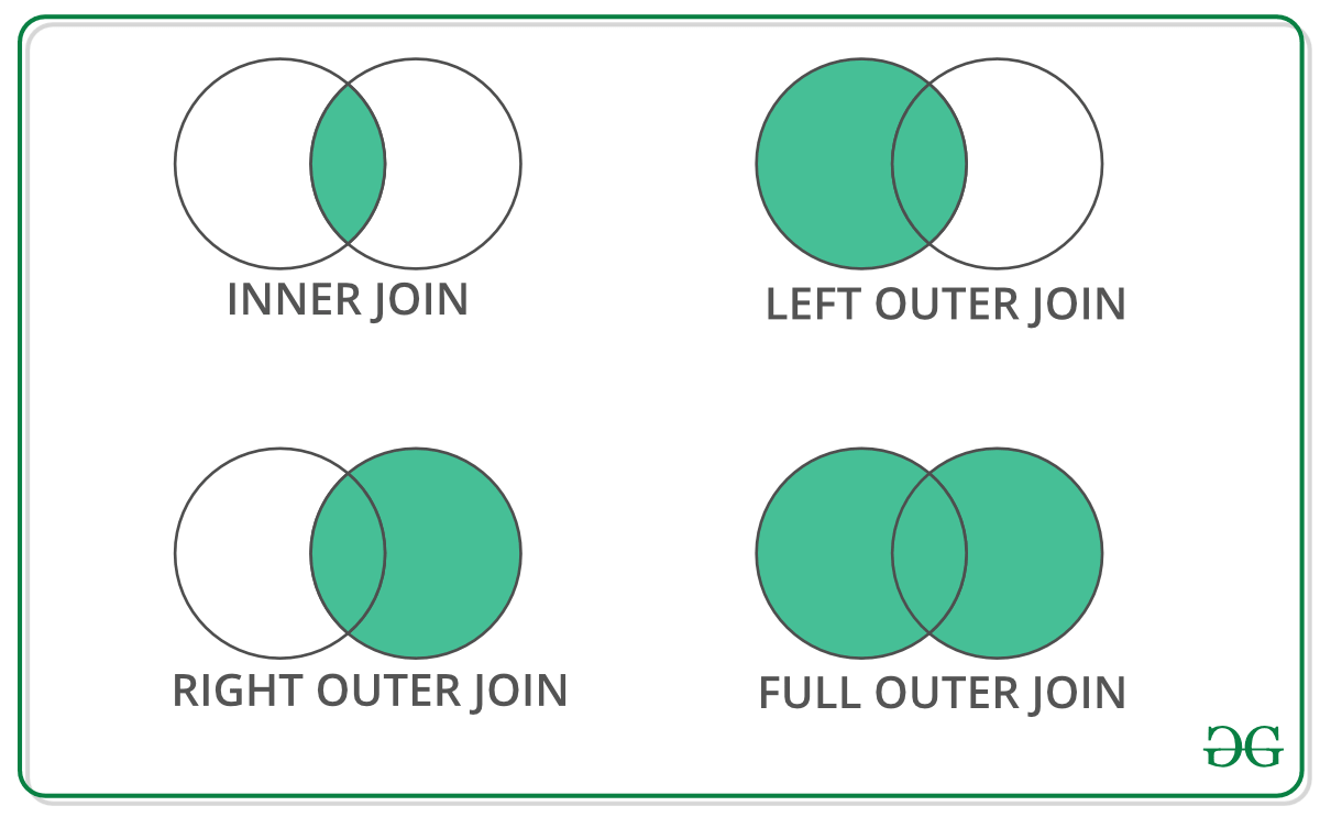
Types of Joins

Creating a Location Metadata Table

# Sensor location metadata (you might get this from a GIS or council database)
sensor_metadata = pd.DataFrame({
    'Location': ['107 Quay Street', '45 Queen Street', '150 K Road',
                 '30 Queen Street', '2 High Street', '61 Federal Street'],
    'Area': ['Waterfront', 'CBD', 'K Road', 'CBD', 'CBD', 'CBD'],
    'Latitude': [-36.8430, -36.8442, -36.8580, -36.8460, -36.8478, -36.8490],
    'Longitude': [174.7685, 174.7659, 174.7560, 174.7665, 174.7670, 174.7620]
})

print(sensor_metadata)

Inner Join

Only keeps rows that match in both DataFrames:

# Merge long-format pedestrian data with location metadata
merged = pd.merge(ped_long, sensor_metadata, on='Location', how='inner')
print(f"Rows in ped_long: {len(ped_long)}")
print(f"Rows after inner join: {len(merged)}")
print(merged.head())

Only locations present in both DataFrames survive an inner join. If sensor_metadata contains only 6 locations, the merged result will only have data for those 6 sensors.

Left Join

Keeps all rows from the left DataFrame:

# Keep ALL pedestrian records, even if we lack metadata for some sensors
merged_left = pd.merge(ped_long, sensor_metadata, on='Location', how='left')
print(f"Rows after left join: {len(merged_left)}")

# Check which locations have no metadata
no_metadata = merged_left[merged_left['Area'].isnull()]['Location'].unique()
print(f"Locations without metadata: {no_metadata}")

Merging with Different Column Names

If the key columns have different names in the two DataFrames, use left_on and right_on:

df1 = pd.DataFrame({
    'sensor_name': ['45 Queen Street', '150 K Road'],
    'daily_avg': [8500, 4200]
})

df2 = pd.DataFrame({
    'location': ['45 Queen Street', '150 K Road'],
    'area': ['CBD', 'K Road']
})

merged = pd.merge(df1, df2, left_on='sensor_name', right_on='location', how='inner')
print(merged)

Practical Example: Enriching Pedestrian Data

# Merge pedestrian data with metadata, then analyse by area
merged = pd.merge(ped_long, sensor_metadata, on='Location', how='inner')

# Average hourly count by area
area_summary = merged.groupby('Area')['Count'].agg(['mean', 'sum', 'count']).round(1)
print("\nPedestrian traffic by area:")
print(area_summary)

# Average hourly count by area and time period
area_period = merged.groupby(['Area', 'Period'])['Count'].mean().round(1)
print("\nTraffic by area and period:")
print(area_period.unstack())

Quick Introduction to Visualisation

Section 2.3 covers visualisation in depth. Here is a preview using the pedestrian data.

Basic Plotting with pandas

import matplotlib.pyplot as plt

# Bar plot: average hourly count by location
location_means = ped[location_cols].mean().sort_values(ascending=False)
location_means.plot(kind='barh', figsize=(10, 8), color='steelblue')
plt.xlabel('Average Hourly Pedestrian Count')
plt.title('Average Hourly Pedestrian Counts by Sensor Location (2024)')
plt.tight_layout()
plt.show()

# Line plot: hourly pattern for a single day
one_day = df[df['Date'] == '2024-03-15']
one_day.plot(x='Hour', y=['queen_st_45', 'k_road_150', 'quay_st_107'],
             figsize=(10, 5), marker='o')
plt.ylabel('Pedestrian Count')
plt.title('Hourly Pedestrian Counts - 15 March 2024')
plt.legend(title='Location')
plt.grid(True, alpha=0.3)
plt.tight_layout()
plt.show()

# Histogram: distribution of hourly counts at Queen Street
df['queen_st_45'].plot(kind='hist', bins=30, edgecolor='black', figsize=(8, 5))
plt.xlabel('Hourly Pedestrian Count')
plt.title('Distribution of Hourly Counts at 45 Queen Street (2024)')
plt.show()

Section 2.3 Goes Deeper

This is just a taste of what is possible. Section 2.3 covers matplotlib for full control over every plot element, seaborn for beautiful statistical graphics, interactive plots with plotly, multi-panel dashboards, and techniques for creating publication-quality figures. For now, use these simple pandas plotting methods to quickly visualise your data during analysis, catching errors and spotting patterns before investing in more polished graphics.

Complete Workflow Example: Auckland Pedestrian Analysis

Let us put everything together in a realistic analysis workflow. This mirrors the kind of analysis an urban planner or transport researcher might conduct to understand pedestrian patterns in Auckland’s city centre.

import pandas as pd
import numpy as np
import matplotlib.pyplot as plt

# ============================
# 1. LOAD DATA
# ============================

url = 'https://raw.githubusercontent.com/dataandcrowd/GISCI343/refs/heads/main/pedestrians/akl_ped-2024.csv'
ped = pd.read_csv(url)

# Drop non-data rows (blank separators and Daylight Savings marker)
ped = ped.dropna(subset=['Date', 'Time'])
ped = ped[ped['Date'] != 'Daylight Savings']
print(f"Data loaded: {ped.shape[0]} rows, {ped.shape[1]} columns")

# ============================
# 2. INITIAL EXPLORATION
# ============================

print("\nColumn names:")
print(ped.columns.tolist())
print(f"\nMissing values:\n{ped.isnull().sum()[ped.isnull().sum() > 0]}")

# ============================
# 3. DATA PREPARATION
# ============================

df = ped.copy()
df['Date'] = pd.to_datetime(df['Date'])
df['Month'] = df['Date'].dt.month
df['DayOfWeek'] = df['Date'].dt.day_name()
df['IsWeekend'] = df['Date'].dt.dayofweek >= 5
df['Hour'] = df['Time'].str.split(':').str[0].astype(int)

# Identify the 20 sensor location columns
location_cols = df.columns[2:22]
df['Total'] = df[location_cols].sum(axis=1)

print(f"\nPrepared data shape: {df.shape}")

# ============================
# 4. TEMPORAL ANALYSIS
# ============================

# Average pedestrian count by hour across all sensors
hourly_avg = df.groupby('Hour')['Total'].mean().round(0)
print("\nAverage total pedestrians by hour:")
print(hourly_avg)

# Weekday vs weekend comparison
weekday_avg = df[~df['IsWeekend']].groupby('Hour')['Total'].mean()
weekend_avg = df[df['IsWeekend']].groupby('Hour')['Total'].mean()

# ============================
# 5. LOCATION ANALYSIS
# ============================

# Rank locations by total annual volume
annual_totals = df[location_cols].sum().sort_values(ascending=False)
print("\nTop 5 locations by annual volume:")
for loc, total in annual_totals.head(5).items():
    print(f"  {loc}: {total:,.0f}")

# ============================
# 6. RESHAPE AND MERGE
# ============================

# Melt to long format for cross-location analysis
df_long = df.melt(
    id_vars=['Date', 'Time', 'Hour', 'Month', 'DayOfWeek', 'IsWeekend'],
    value_vars=location_cols,
    var_name='Location',
    value_name='Count'
)

# Average by location and whether it is a weekday or weekend
location_comparison = df_long.groupby(['Location', 'IsWeekend'])['Count'].mean().unstack()
location_comparison.columns = ['Weekday', 'Weekend']
location_comparison['Ratio'] = (location_comparison['Weekend'] / location_comparison['Weekday']).round(2)
print("\nWeekend-to-weekday ratio by location:")
print(location_comparison.sort_values('Ratio', ascending=False))

# ============================
# 7. VISUALISATION
# ============================

fig, axes = plt.subplots(2, 2, figsize=(14, 10))

# Plot 1: Average hourly pattern (weekday vs weekend)
axes[0, 0].plot(weekday_avg.index, weekday_avg.values, marker='o', label='Weekday')
axes[0, 0].plot(weekend_avg.index, weekend_avg.values, marker='s', label='Weekend')
axes[0, 0].set_title('Average Hourly Pedestrian Counts', fontweight='bold')
axes[0, 0].set_xlabel('Hour of Day')
axes[0, 0].set_ylabel('Total Count (all sensors)')
axes[0, 0].legend()
axes[0, 0].grid(True, alpha=0.3)

# Plot 2: Top 10 locations by annual volume
top_10 = annual_totals.head(10)
top_10.plot(kind='barh', ax=axes[0, 1], color='steelblue')
axes[0, 1].set_title('Top 10 Locations by Annual Volume', fontweight='bold')
axes[0, 1].set_xlabel('Total Annual Count')

# Plot 3: Monthly trend
monthly_total = df.groupby('Month')['Total'].sum()
monthly_total.plot(kind='bar', ax=axes[1, 0], color='forestgreen')
axes[1, 0].set_title('Total Pedestrian Counts by Month', fontweight='bold')
axes[1, 0].set_xlabel('Month')
axes[1, 0].set_ylabel('Total Count')

# Plot 4: Distribution of hourly counts at the busiest location
busiest_location = annual_totals.index[0]
df[busiest_location].plot(kind='hist', bins=30, ax=axes[1, 1],
                           edgecolor='black', color='coral')
axes[1, 1].set_title(f'Hourly Count Distribution: {busiest_location}', fontweight='bold')
axes[1, 1].set_xlabel('Hourly Count')

plt.tight_layout()
plt.show()

# ============================
# 8. EXPORT RESULTS
# ============================

# Save the enriched dataset
df.to_csv('auckland_pedestrian_enriched.csv', index=False)

# Save location summary
annual_totals.to_csv('location_annual_totals.csv')

print(f"\nAnalysis complete.")
print(f"Total sensor-hours analysed: {len(df):,}")
print(f"Total pedestrian counts recorded: {df['Total'].sum():,.0f}")
print(f"Busiest location: {annual_totals.index[0]}")
print(f"Busiest month: month {monthly_total.idxmax()}")

Summary

This section has taken you through the complete pandas workflow, from raw data to analytical insight, using Auckland’s real pedestrian count data as the throughline. You began with dictionaries, Python’s key-value data structure that underpins GeoJSON and API responses, and the gateway through which most real-world geospatial data enters your analysis pipeline. You then learned how to create DataFrames from dictionaries and read real data from CSV files, each with their own set of import arguments for handling headers, data types, and missing values.

Exploring DataFrames through methods like .describe(), .info(), .head(), and .tail() gives you the initial understanding of your data’s structure, size, and quality. Selecting and filtering data, whether through column selection, .iloc[]/.loc[] indexing, boolean indexing, or the .query() method, allows you to isolate the records and variables relevant to your analysis. The .copy() method ensures that your filtered subsets do not inadvertently modify the original data.

The groupby operation, which follows the split-apply-combine pattern, is perhaps the single most important analytical tool in pandas for geospatial work. Whether you are computing average pedestrian counts by hour of day, total volumes by sensor location, or weekday-vs-weekend ratios across the city centre, groupby is the mechanism that makes this possible. Pivot tables and melting operations complement groupby by reshaping data between wide and long formats, each suited to different analytical and visualisation tasks.

You also addressed the reality of messy data by learning to detect, remove, and fill missing values, and you combined datasets through merge operations (inner, left, right, and outer joins) that directly parallel the spatial joins you will learn in Section 2.4. Finally, a preview of pandas’ built-in plotting capabilities demonstrated how quick visualisations can verify your data processing at each stage of an analysis.

Connection to Other Sections

This section sits at the centre of Part 2’s learning arc. From Section 2.1, you brought forward lists (which became DataFrame columns), for loops (used to iterate through DataFrames and dictionaries), and conditionals (which power boolean indexing and the .apply() method). Moving forward to Section 2.3, everything you have learned about data manipulation feeds directly into visualisation. The groupby results you computed here become bar charts and line plots; pivot tables become heatmaps; filtered subsets become the data behind scatter plots. Looking ahead to Section 2.4, the transition from pandas to geopandas is remarkably smooth because a GeoDataFrame is simply a pandas DataFrame with an additional geometry column. Every filtering, grouping, merging, and reshaping operation you have mastered here transfers directly to spatial data analysis. Indeed, the sensor location metadata you merged with the pedestrian counts is precisely the kind of operation that becomes a spatial join once you add coordinates and geometry.

Key Takeaways

Essential Skills for GIS Analysis

The six pandas skills that matter most for geospatial work are:

dictionaries (they underpin GeoJSON and APIs)
groupby (summarise anything by zone or category)
boolean indexing (filter by attributes)
merging (the tabular version of spatial joins),
handling missing data (sensors fail, surveys have gaps)
visualising early and often (catch errors before they propagate).

Practice Exercises

Exercise 1: Dictionary to DataFrame

Create a dictionary containing metadata for five Auckland pedestrian sensor locations (name, latitude, longitude, area). Convert it to a DataFrame. Calculate the distance of each sensor from a reference point (e.g. Britomart Transport Centre at -36.8442, 174.7680) using the Euclidean distance formula. Which sensor is closest?

# Your code here
# Step 1: Convert to DataFrame
df = pd.DataFrame(sensors)

# Step 2: Define reference point (Britomart)
ref_lat = -36.8442
ref_lon = 174.7680

# Step 3: Calculate Euclidean distance for each sensor
df['distance'] = np.sqrt(
    (df['latitude'] - ________)**2 +  # quiz 3
    (df['longitude'] - ________)**2   # quiz 3
)

# Step 4: Find closest sensor
closest = df.loc[df['distance'].idxmin(), 'name']

print(df[['name', 'distance']])
print(f"\nClosest sensor to Britomart: {closest}")

Exercise 2: Exploring the Pedestrian Data (ungraded, but worth trying)

Load the Auckland pedestrian data and answer these questions:

How many rows and columns does the dataset have?
Which location has the highest single-hour count in the entire year?
What percentage of values are missing across the whole dataset?
What is the average hourly count at each location?

Exercise 3: Filtering and Temporal Analysis (ungraded, but worth trying)

Using the pedestrian data:

Filter for only weekend data (Saturday and Sunday)
Filter for the evening peak (17:00-18:59)
Find all hours where 45 Queen Street had more than 1000 pedestrians
What day of the year had the highest total pedestrian count across all sensors?

Next Steps

You now have the data manipulation skills to load and clean data, filter and group records, calculate new metrics, and combine datasets from multiple sources.

The Auckland pedestrian data you worked with here will continue to appear in Section 2.3 (Visualisation), where you will learn to create publication-quality plots with matplotlib and seaborn, and in Section 2.4 (GeoPandas), where you will add the spatial dimension by geocoding the sensor locations and performing spatial analysis.

The pandas skills you have learned transfer directly, because GeoPandas is fundamentally pandas with geometry.

Sevtsuk, Andres, and Raul Kalvo. 2024. “Modeling Pedestrian Activity in Cities with Urban Network Analysis.” Environment and Planning B: Urban Analytics and City Science. https://doi.org/10.1177/23998083241261766.

Introduction

Dictionaries: Flexible Data Structures

What is a Dictionary?

Creating Dictionaries

Dictionary Methods

Iterating Through Dictionaries

Nested Dictionaries

Why Dictionaries Matter for GIS

Practical Example: API Response

Packages and Imports

Installing Packages

The import Statement

Standard Aliases

Getting Started with Pandas

What is pandas?

Import

Creating DataFrames

What is a DataFrame?

From a Dictionary (The Key Connection!)

From a List of Dictionaries

Reading the Auckland Pedestrian Data

Reading a CSV File

Other File Formats

Saving DataFrames

Exploring the Pedestrian Data

Initial Inspection

DataFrame Properties

Data Types

Information Summary

Summary Statistics

Selecting Data

Selecting Columns

Selecting Rows by Index

Boolean Indexing (Filtering)

Filtering by Date and Time

The .query() Method

Copying DataFrames

Manipulating Data

Creating New Columns

Conditional Column Creation

Modifying and Renaming Columns

Grouping and Aggregation

Basic Grouping

Multiple Aggregations

Aggregating Multiple Columns

Grouping by Multiple Variables

Custom Aggregation Functions

Practical Example: Monthly Pedestrian Volumes

Reshaping Data

Melting (Wide to Long)

Pivot Tables (Long to Wide)

When to Use Which Format

Handling Missing Data

Detecting Missing Data

Removing Missing Data

Filling Missing Data

Best Practices

Merging DataFrames

Types of Joins

Creating a Location Metadata Table

Inner Join

Left Join

Merging with Different Column Names

Practical Example: Enriching Pedestrian Data

Quick Introduction to Visualisation

Basic Plotting with pandas

Complete Workflow Example: Auckland Pedestrian Analysis

Summary

Connection to Other Sections

Key Takeaways

Practice Exercises

Further Reading

Next Steps

The `import` Statement

The `.query()` Method